Complete guide to classification algorithms

Classification is the task of predicting a class based on the available data. It is a common and useful problem in many areas, such as medicine, marketing, and banking. A simple example of a classification problem that you face daily is email. The types of classification algorithms in machine learning classify your emails as spam, or not. It is a binary classification. There are several types of classification algorithms in machine learning:

1. Binary Classification
2. Multi-Class Classification
3. Multi-Label Classification
4. Imbalanced Classification

In this article, we’ll take a look at classification types in machine learning. We’ll deal with binary classification and imbalanced classes simultaneously. 

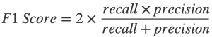
The following structure applies to all data science concept in the article. The first step is to determine the classifier. The second is to train the model. At this stage, the classifier fits data with features and its class label.  The model learns all types of machine learning algorithms from previously known data and its categories. Therefore, the task using types of machine learning classification is supervised learning. The classifier tries to establish relationships between the input features and their class. You can proceed to the prediction of new data after model training. And the last step is to check the quality of the tuned algorithm. The F1 Score is a metric for evaluating the performance of the model’s harmonic mean. It has the following calculation formula:

We will also build the confusion matrix by class to check the distribution of predictions between classes.

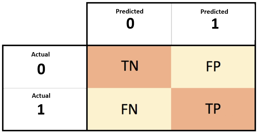Representation of a confusion matrix (source)

The processing time is another crucial parameter for analyzing the types of classification algorithms. 

In the article, we will consider the following 4 machine learning classification types and their implementation in Python:

• Logistic regression
• Naive Bayes
• Support Vector Machines (SVM)
• Random Forest

What is classification in Machine Learning?

Classification is one of the basic approaches in machine learning that helps a computer make data-driven decisions. Simply put, the classification algorithm receives input and determines which category it belongs to.

Examples from business:

– In the bank, the algorithm classifies the client as reliable or risky

– In medicine – determines whether there is a possibility of disease

– In e-commerce – recognizes whether a person will respond to a promotion

Machine learning does not replace employees – it automates everyday tasks where many solutions of the same type are required. This improves accuracy, speeds up processes, and reduces costs.

If you are considering implementing ML models, a reliable machine learning company will help you quickly launch a solution for your task. There is no need to immediately build an internal team: experienced contractors speed up the start and help avoid mistakes.

Types of classification problems

There are several main types of classification that companies in different industries use:

Binary classification

– Only two classes: yes/no, will/will not, positive/negative

– Examples of machine learning algorithms: spam detection, fraud checking, churn prediction (will the client leave)

Multi-class classification

– More than two categories

– Examples: automatic determination of product category, recall key (positive/neutral/negative), document type

Multi-label classification

– An object can belong to several categories at once

– Example: e-mail can be both important and requiring a response

The choice of approach depends on the task and the available data. A well-chosen classification type reduces manual labor costs, speeds up analytics and improves the quality of service.

How classification algorithms make decisions

Classification algorithms are trained on examples. First, they are given historical data: what was at the entrance and what result was correct. Based on these examples, the model “learns” to find patterns.

After training, the algorithm applies these patterns to new, not yet seen data – and determines which category they belong to.

In simple words: if you have a history of orders, the model will be able to predict which client to offer this or that product. Or automatically recognize cases that require priority, for example, complaints or risks.

The larger and cleaner the data, the more accurate the model. But the key is not the volume, but the competent formulation of the task and business goals. This is where we always start projects at Data Science UA.

Popular classification algorithms

There are dozens of classification algorithms. The following are the most commonly used in business practice:

Logistic regression

A simple and efficient way of binary classification. Good for MVP and quick starts.

Decision trees и random forests

Clear and visual models. Used for tasks where interpretability is important (e.g. fintech, HR, compliance).

Support vector machines (SVM)

Work well with a small amount of data with clearly separable classes.

Gradient boosting (XGBoost, LightGBM, CatBoost)

Powerful ensembles that show high accuracy in complex tasks. Suitable for advanced solutions.

Neural networks

Used for complex unstructured data (images, texts). CV and NLP solutions work on their basis.

Choosing a model is not about being “fashionable”. This is about how it fits specific business conditions: speed, accuracy, interpretability, support in sales.

Dataset

The Bank Marketing Data Set is a dataset from the UCI Machine Learning Repository. The data was collected through calls to customers (features job, education, loans, etc.). The goal is to predict whether a client will subscribe to a term deposit or not (label y). 

The dataset has 41,188 rows, 20 feature columns, and one target column. Label y has two values, “yes” (1) and “no” (0). This means the classification is binary. The majority of y values is 0, so we are dealing with imbalanced classes.

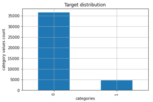y column label distribution

Some of the columns are categorical. These columns are converted to numerical form before using the machine learning classification algorithms (by LabelEncoder). It’s good to standardize the dataset for optimalmodel performance (by StandardScaler). Additionally, we define a weight variable that will correspond to the inversely proportional distribution of y classes:

w = {0:11, 1:89}

The weight will be assigned to the labels for the models’ training due to unbalanced classes. Next, we will look at and apply some of the best classification algorithms.

Logistic Regression

Logistic regression is one of the most basic and standard methods to tackle data related challenges in machine learning. These types of machine learning classification seek to find the most appropriate relationship between a target variable and a set of independent variables. This algorithm is similar to Linear Regression with additionally using a logistic function. Thus, an observation belongs to one of the classes with a probability of 0.5. The line separating the two classes has an S form.

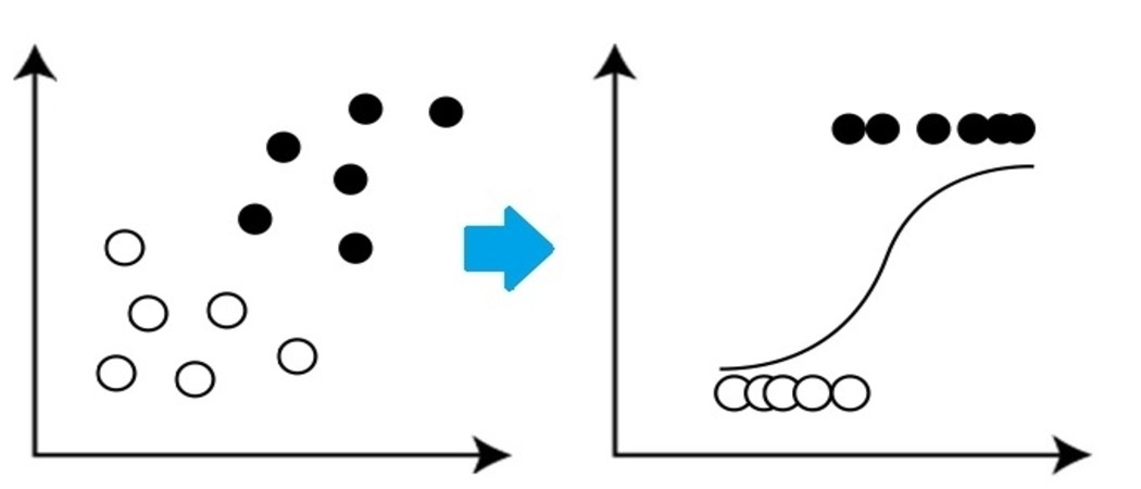Logistic regression line separating classes (source)

Advantages. This classifier is a pretty simple algorithm with high efficiency. It calculates the probabilities of an observation assigned to a class. 

Disadvantages. The algorithm works only for binary all classification algorithms in machine learning. All predictors are assumed to be independent of each other.

Python realization of a Logistic regression for our bank dataset:

The distribution of right predicted observations and incorrectly is seen using the confusion matrix. The first line corresponds to class “0” labels. 6,189 observation marks are proper, but 1,105 are not. Class “1” is in line 2 with reverse order. 826 marks are correct, but 118 are not. Note that the model predicted most of the observations of each class properly. We will compare the F1 score and time between all models in the score table at the end.

Naive Bayes

This algorithm is the classifier based on the Bayes’ theorem. All predictors are assumed to be independent of each other by such machine learning classification types. The presence of each feature and its values doesn’t depend on other columns in the dataset. 

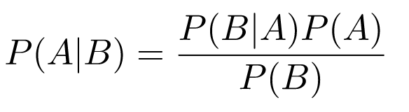Bayes’ theorem (source)

P(A|B) is the probability of event A occurring when event B occurs.
P(B|A) is the probability of event B occurring when event A occurs.
P(A) / P(B) is the probability of event A / B occurring.

Gaussian Naive Bayes are a machine learning classification techniques based on Naive Bayes and the data binomial (normal) distribution.

Advantages. The machine learning classification techniques work well even with a small dataset. It works fast compared to other classifiers.

Disadvantages. The classifier works well with independent features. It is not very common in the real world.

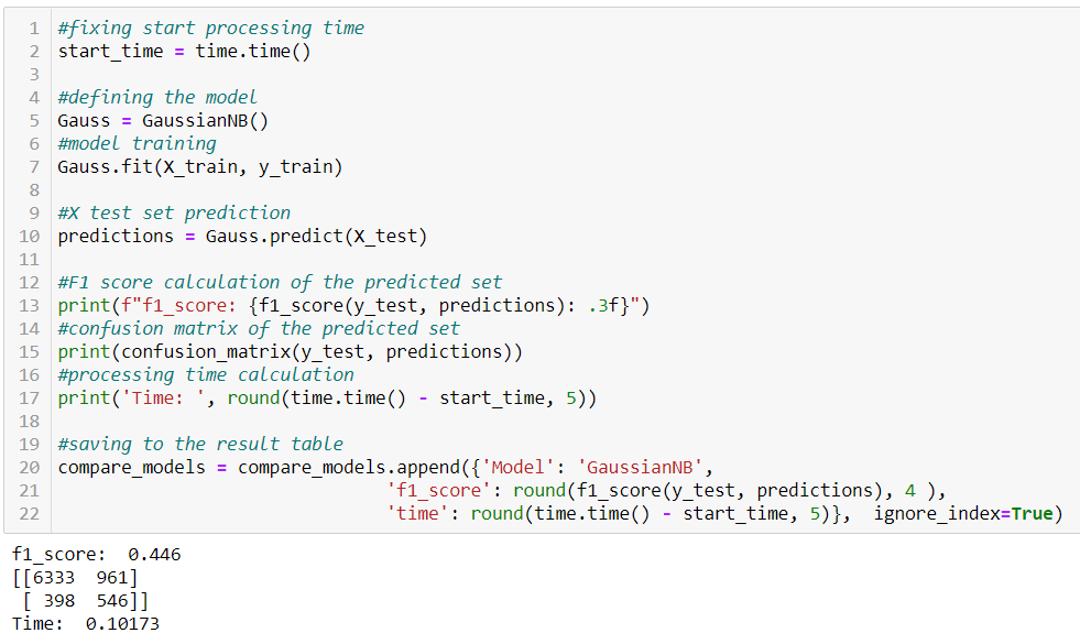
Python realization of Naive Bayes for the bank dataset:

As before, the model correctly predicted most class labels “0” and “1”. Let’s compare the distribution of categories with Logistic Regression. The predictions have improved for class “0” by almost 150 observations. But label “1” was predicted much worse by nearly 300. Taking into account the unbalanced classes, this influenced the decrease of the F1 metric. Note that Gaussian Naive Bayes in Python doesn’t have a hyperparameter for class weights like other types of machine learning classification from this article.

Support Vector Machine (SVM)

SVM is an algorithm for regression and classification problems that has contributed significantly to the achievements of artificial intelligence. The concept is to find a hyperplane that separates the points into different categories. The points in space represent training data. The points from one class should be separated from another class by the broadest possible distance. This distance is called margin. New data is similarly transformed into points in this space. They will be marked with the appropriate label depending on which side of the hyperplane they are on.

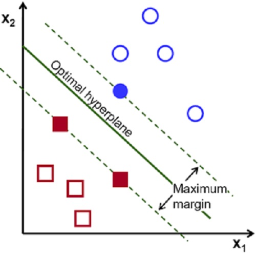SVM space with optimal hyperplane (source)

Advantages. The algorithm is efficient in high-dimensional spaces. It works well when there is a clear margin between the categories. 

Disadvantages. Noise in the dataset degrades the result. SVM is not suitable for large datasets.

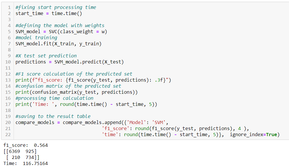
Python realization of SVM for the bank dataset:

Like previous algorithms, the SVM predicted most of the observations in each class correctly. It is between Logistic Regression and Naive Bayes by valid mark quantity of each category according to the confusion matrix. An important point is the model’s running time. It is several hundred times larger than previous algorithms.

Random Forest

Random Forest doesn’t belong to basic types of machine learning classification algorithms. It is an ensemble of several Decision Trees combined into one algorithm. So first, let’s discuss the Decision Tree method.

This algorithm solves both classification and regression problems and is used by machine learning software development services. The model builds a form of a tree structure and creates a sequence of rules. Step by step, the original dataset is split into smaller and smaller subsets by these rules. So, an associated decision tree appears with decision nodes and leaf nodes. The algorithm simulates human thinking, and you can easily follow the logic.

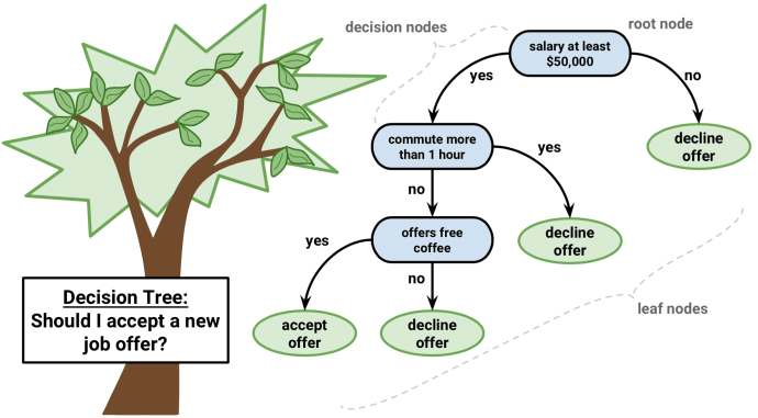Decision tree example with nodes (source)

The ensemble of Decision Trees increases the predictive power over the independent one. The Random Forest combines them for better results. Deep trees can have an overfitting problem. Therefore, Random Forest creates trees on random subsets of the dataset, which eliminates the issue of overfitting. Finally, all trees vote to make the prediction decision.

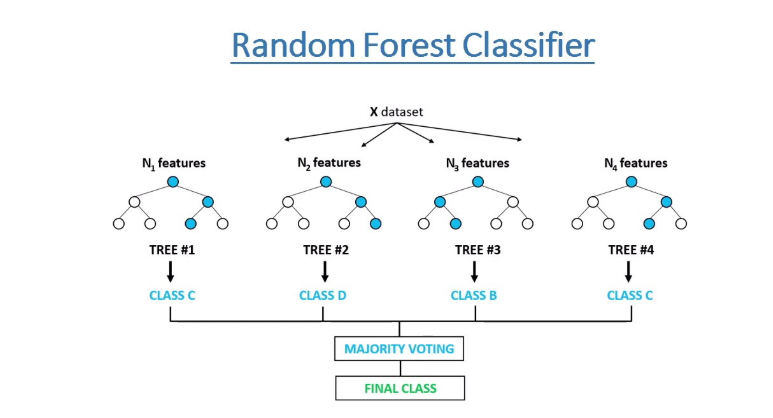Representation of Random Forest algorithm (source)

Advantages. It is a more accurate algorithm than the Decision Tree and is much less subject to overfitting. Rules make decisions, so this method works with categorical and continuous data, missing values, and the dataset does not need to be normalized.

Disadvantages. A Random Forest consists of many trees, so it requires more computing power and more training time. It slows down a real-time prediction. Also, the model can be complex to implement due to many hyperparameters selection.

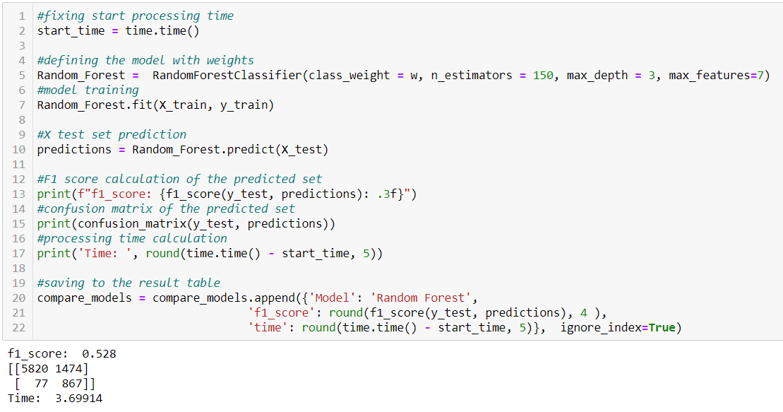
Python realization of Random Forest for the bank dataset:

The ensemble of Decision Trees singled out and predicted class “1” very well. The classifier has the most accurate result in this category compared to previous ones. In contrast, Random Forest predicted class “0” worst of all. It completed the task much faster than SVM but still a little slower than the first two algorithms. This is because the classifier is an ensemble of trees.

K-Nearest Neighbor overview

K-Nearest Neighbor (K-NN) is one of the most popular classification methods in machine learning. It is a type of supervised learning algorithm that can be used for both regression and classification tasks. In this article, we will provide an overview of K-NN, one of the best machine learning algorithms for classification.

The K-NN algorithm works by selecting the number of nearest neighbors (K) for each data point, calculating the distance between the data points and their neighbors, and assigning the class of the majority of the K-nearest neighbors to the new data point. The distance measure used can be Euclidean, Manhattan, or Minkowski distance.

One of the strengths of K-NN is that it can work well with both small and large datasets. It is a non-parametric algorithm, meaning it does not make assumptions about the underlying data distribution. Moreover, K-NN does not require training on the data, and it can be used for both binary and multi-class classification problems.

However, K-NN has some limitations. It can be sensitive to noisy or irrelevant features, and it can also suffer from the curse of dimensionality. Additionally, K-NN can be computationally expensive for large datasets since it requires calculating the distance between each data point and all the other data points.

Despite these limitations, K-NN remains one of the best machine learning algorithms for classification. It has been used in a wide range of applications, including image recognition, text classification, and anomaly detection.

In summary, K-NN is a simple and effective algorithm that can be used for classification tasks in machine learning. It is a non-parametric algorithm that can work well with small and large datasets, and it can be used for both binary and multi-class classification problems. Although it has some limitations, it remains one of the best machine learning algorithms for classification.

K-Nearest Neighbor code

Implementing K-NN in code is relatively straightforward. One can use various libraries like scikit-learn, TensorFlow, and PyTorch to implement the K-NN algorithm.

For instance, scikit-learn is a popular machine learning library that provides KNeighborsClassifier class to implement K-NN in Python. Below is a code snippet that demonstrates how to create and predict with a KNN model using scikit-learn:

In the above code, “n_neighbors” specifies the number of neighbors to consider, “metric” specifies the distance measure to use, and “p” is the power parameter for the Minkowski distance. Once the model is created, it can be trained on the training data using the “fit” method and can be used to predict the labels for the test data using the “predict” method.

Overall, implementing K-NN in code using libraries like scikit-learn is simple and easy. With the availability of these libraries, K-NN has become one of the best machine learning algorithms for classification tasks in machine learning.

Gradient Boosting Algorithms (XGBoost, LightGBM, CatBoost)

Gradient Boosting is a method that combines many weak models (usually decision trees) to get a strong one. Each new “booster” corrects the errors of the previous ones. Algorithms of the gradient boosting family are among the most popular in practice today.

Why businesses should pay attention:

• High accuracy and stability on real data.
• Universality: can be applied to table data, time series, tasks with a weakly expressed structure.
• Support for categorical features (especially CatBoost).
• Robustness to missing values and unbalanced samples.

Where used:

• Fintech: scoring, risk assessment, anti-fraud.
• Marketing: outflow prediction, personalization of offers.
• E-commerce: recommendations, dynamic pricing.

Why implementation experience matters:

Even a powerful algorithm can “sink” if the data or metrics are incorrectly prepared. Therefore, it is important to work with a team that can build an end-to-end ML system – from data pipeline to business integration.

Neural networks for classification

Neural networks are universal architectures that mimic the work of the human brain. Unlike basic ml algorithms, they can find complex, non-linear dependencies in data. This makes them especially useful for unstructured data: images, audio, text.

What you need to know:

1. Neural networks require more data and resources.
2. But they often outperform common machine learning models in quality on complex tasks.
3. Harder to interpret. For some industries (medicine, finance), this can be critical.

Where applicable:

• Medicine: classification of MRI images, X-rays, disease prediction.
• Retail and e-commerce: visual search, analysis of user behavior.
• Security: facial recognition, identifying suspicious objects on video.
• Customer support: understanding of texts, chatbots based on intent classification.

Modern approaches to classification in Machine Learning

Modern classification approaches make it possible to increase the accuracy of models, speed up their training and simplify interpretation. These methods are increasingly becoming part of real solutions when reliability and scalability are important to business.

If you are planning to implement such solutions, it is important to assess which approach will suit your task. AI consulting will help with this – an audit and recommendations for choosing the best models, infrastructure and processes.

Deep ensemble methods

Ensembly is an approach where multiple models are combined into one stronger one. Deep ensembles use neural networks as basic models. This approach is resistant to retraining and can take into account different aspects of the data.

For example, an insurance company predicts the risk of refusing to pay. One algorithm focuses on customer data, another on case history, and a third on user behavior. Their combination gives a stable result, important for making decisions in high-risk zones.

XAI Techniques

Explainable AI (XAI) are tools that make model behavior understandable to humans. Especially relevant for sensitive industries: medicine, finance, jurisprudence.

Example: the bank uses a model for scoring loans. XAI explains why the client was refused. It reduces legal risks and improves user trust.

Transformers for classification

The architecture of transformers (for example, BERT, RoBERTa) has shown excellent results in text classification problems. They know how to take into account context, sentence structure and even tonality.

For example, in support, case classification helps you quickly route messages to the right operator. Transformers determine exactly where we are talking about a complaint, and where – about an error in delivery, even if the user writes informally.

Comparative analysis of models

The choice of model affects not only accuracy, but also the cost of implementation, the speed of output to production, and the complexity of support.

Key metrics we analyze as an artificial intelligence development company:

• Precision and recall;
• Learning and forecasting time;
• Resistance to unbalanced data;
• Scalability

Such an analysis helps to choose not the “smartest” model, but the optimal one for a specific case: logistics, financial analytics, HR.

Where classification is used in real life

Classification is not a theory. These are specific tasks that occur daily:

• Finance: anti-fraud, risk assessment, scoring applications;
• E-commerce: recommendations, feedback analysis;
• Health care: diagnosis of diseases by images and symptoms;
• Marketing: churn prediction, customer segmentation;
• Industry: analysis of product defects in the photo.

All these solutions require good models, high-quality data preparation and thoughtful business integration. Therefore, it is important to work with a data science development firm, which has experience in building such end-to-end solutions.

If you are thinking where to start, or have already tried to implement ML, but have not seen the ROI, we will discuss your case and show you how to do better.

Comparative analysis. Conclusion

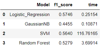
All algorithms classified most of the observations correctly in each class. However, they all had different results, more accurately predicting  class “0” or “1” as we have seen in confusion matrices. It influenced the value of the F1 metric for each classifier. 

Summary table:

Let’s visualize these parameters.

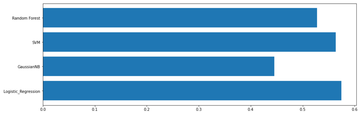
F1 score of classifiers

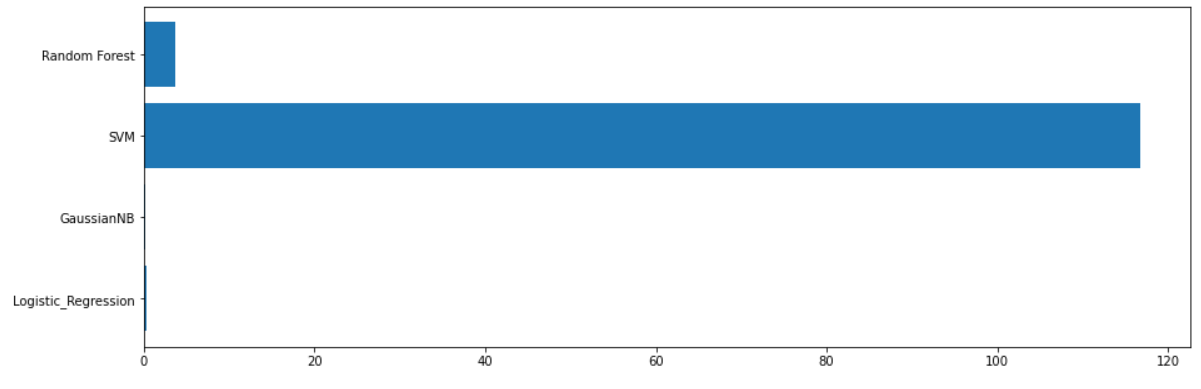Processing time of classifiers

The table and graphs show that the Logistic Regression and SVM have the best results in classifying both categories according to the F1 score. Logistic Regression is much faster than SVM according to the time parameter. Finally, Logistic Regression became the most optimal classifier for The Bank Marketing Data Set.

It is important to note that Logistic Regression is not the best classification algorithm in machine learning for all cases. Each problem is individual, has specific features in the datasets and its own goals. You can analyze data and use different machine learning classification algorithms. Evaluating the model performance determines the appropriate classifier using metrics. 

There are many more other types of machine learning classification for solving the classification problem. In this article, we have covered the most basic and popular methods. But there are still many classifiers for your research.

FAQ