An Intuitive Explanation of Data Science Concepts

Welcome to the part of the series “An Intuitive Explanation of Data Science Concepts.” In the first two articles, we discussed basic DS-related terms and mathematical concepts. In this article, we will concentrate on statistics – one of the most crucial sciences used in data science. 

Statistics provides several vital techniques and approaches that are widely used when working with data. It allows us to extract meaningful trends and changes, discover hidden patterns and insights, describe the data, and create relevant features.

All of these turn out to be crucial for any data scientist. So let’s not waste time and get right into it!

Table of contents:

• Basic terms
• Distributions
• Central Limit Theorem
• Hypothesis testing
• Conclusion
• FAQ

Basic Terms

Before going any further, it is crucial to understand the essentials. So, here are a few of the most fundamental concepts in statistics:

A population is an entire group of elements we study. It could be, for example, all the people in a country, or all the cars produced in a factory.

A sample is a subset of a population, a representative in research. For instance, if we want to study a country’s entire population, a sample includes all those who participated in a survey. If we analyze whether a batch of cars has defects, a sample consists of those several cars we take for an examination.

A sample is a representative subset of a population, which consists of randomly chosen elements (source)

Mean is the average value in at dataset. It is calculated as the sum of all values, divided by the number of these values in our data.

Median is the middle value of the ordered dataset. If we have a sorted array of values, the element right in the middle would be the median. If we had an array with an even number of elements (meaning that there are two values in the middle), the median would equal the average of these two values in the middle.

Mode is the most common value in the dataset. For example, if we had a dataset of all fast-food restaurants globally, Subway would be the mode because it has the highest number of locations (41600 as of 2020).

Variance is the measure of dispersion. It shows how the data is spread out with respect to the average value. Variance is calculated by dividing the sum of the differences between each data point and their mean by the number of data points.

Variance definition (source)

Here, σ2is the variance, μ is the mean of the dataset, ✗ is a single data point, ⅀ is the sum, N is the number of observations in the dataset.

Standard deviation is also a measure of dispersion. It is calculated as the square root of variance. But, unlike variance, it is expressed in the same units as the data itself. 

To deepen our knowledge, let’s try to describe a simple dataset with all the concepts above. Consider, for example, the following case: there is a small group of people learning Spanish. The course is coming to an end, and every participant needs to take the final exam. After grading, the following marks were obtained (out of 100): 89, 56, 72, 95, 78, 64, 72, 86, and 90. This will be our sample data.

There are nine people in the group (that is, N = 9). 

The mean (or average) equals: 

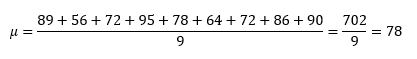The mean is calculated as the sum of all observed values divided by the number of observations

To find the median, we first need to sort our array. We get: 56, 64, 72, 72, 78, 86, 89, 90, 95. There are only nine values, so the middle one (the fifth one) is the median. And it is equal to 78.

The mode is the most frequent value in the dataset. We can see each number only once, except for the 72 (which appears twice). So, the mode equals 72. In the case of multiple numbers appearing in the dataset an equal number of times, there might also be several modes.

The variance is calculated as follows: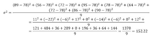

To calculate the variance, you need to subtract the mean from each of the observed values, take the squares of these differences, sum the results up, and divide by the number of observations

Finally, to calculate the standard deviation, we need to take the square root of the variance, which equals 12.458.

Distributions

Let’s now move on to the next important topic – probability distributions. A probability distribution is simply a function that assigns probabilities to possible outcomes of an experiment. The definition can also be formulated as follows: the distribution of a variable describes the number of times each outcome will occur in a certain number of trials. 

We never know for sure what the result of the experiment will be. However, we have certain expectations. For example, when flipping a coin, we can expect it to turn heads in approximately 50% of trials. And that is precisely what a probability distribution describes.

There are various distributions, each used for different scenarios. But all distributions can be divided into discrete and continuous. Discrete distributions are used for experiments that have a limited number of possible outcomes. Consider the example of throwing a fair die. There are only six possible outcomes. Such experiments should be described with discrete distributions. On the other hand, continuous distributions serve to describe experiments with infinitely many outcomes. For example, when you throw a ball, it may reach precisely 50 meters, or 50 meters and 7 centimeters, or 50 meters, 7 centimeters, and 2 millimeters, and so on. There are infinitely many possible outcomes, and the probability of each individual one equals zero. Therefore, continuous distributions are used instead of the usual probability.

Again, there are many distributions with different purposes. Some of the most widely used discrete distributions are Bernoulli, binomial, and Poisson. The most popular continuous distributions include uniform, exponential, and normal (or Gaussian) distributions. The normal distribution is fascinating. Let’s discuss it a bit more deeply. 

This distribution is widely used in natural and social sciences and has several valuable properties. It has a bell-shaped curve, as shown below. It can be seen from the figure that the closer the event is to the mean, the higher is its probability. On the other hand, if an event is far from the mean, its probability is minuscule. The importance of the normal distribution is partly due to the Central Limit Theorem, which will be covered a bit later in this article. Still, the main reason why normal distribution is so important is that it fits many natural phenomena. Human heights, animal population, blood pressure, students’ grades, and many other statistics can be described with Gaussian distribution.

The normal distribution has a typical bell-like shape (source) 

Central Limit Theorem

The Central Limit Theorem (CLT) is probably one of the most important ones in statistics. It states that having a sufficiently large number of samples from a population, sample means will be approximately normally distributed. That is, if you have, say, a thousand samples taken randomly from a population, for each of these samples you calculate the mean, then all these means will approximately have Gaussian distribution. 

Why is it so important? The central limit theorem basically allows us to use a normal distribution for many tasks and problems, even for those that deal with other types of distributions. In other words, even if you don’t know what statistical distribution your data has, you can use normal distribution provided that you have enough data. And, as you may already know, the normal distribution is very convenient to work with. 

The central limit theorem explains many real-world phenomena: from the distribution of lottery winnings to electric noise. 

We will not prove the central limit theorem here, as it is an article with intuitive explanations, not mathematical proofs. But you can easily test the CLT using a bit of statistics or programming knowledge (just like in this article). 

Hypothesis Testing

We are finally arriving at the most crucial topic in statistics – hypothesis testing. 

Hypothesis testing is precisely what it sounds like – it is the process of checking whether a specific statement (hypothesis) is true based on the observed data. 

Let’s look at the example. Suppose you are a math teacher, and you have a class of thirty students. The average mark on the last exam was 61 points out of 100. This is a pretty low grade, isn’t it? And you now think: is the new generation really so bad at math? 

This might be an example of a hypothesis. And the process of testing is called hypothesis testing. Pretty simple, right? In our specific example, during the hypothesis testing process, you will try to figure out, whether all students are bad at math or it is just a coincidence that your class received such marks (there is also a possibility that you are not the best teacher, but for the sake of this article we will conclude that you are a great one😁)

Now, there are several methods used for hypothesis testing. The most popular one – p-value – is discussed in detail in our other article. So here, let’s just briefly look at the typical process of hypothesis testing.

It usually consists of the following steps: 

1. Formulating the null and alternative hypotheses
2. Determining the properties of the test: the size of the sample, the significance level, and the type of the hypothesis test (one- or two-tailed)
3. Calculating the test statistic/p-value/confidence intervals (depending on the method chosen)
4. Conducting the test (comparing test statistics with a threshold value)
5. Rejecting or not rejecting the null hypothesis

Since this article provides only intuitive explanations, we will not go too deep in detail. But check out the article about p-values. Most of the concepts mentioned above are explained there in greater detail.

Hypothesis testing is not only a statistical concept. It is widely used in data science as well. It allows us to conclude the population distribution based on the sample data, which is beneficial for data preparation and model selection. It can also help us in feature selection by choosing the best variables out of the available ones. There are many other ways to use hypothesis testing in data science, and you most certainly will encounter them. But don’t worry, you will be ready!

Conclusion

In this article, we have only slightly scratched the surface of statistics. It is an expansive science that can’t be fit into one article. However, we have discussed several important topics that will make your further learning much easier. 

Be sure to check out this article about hypothesis testing with the p-value and this article where we go over some of the discussed concepts with Python. In subsequent articles, we will concentrate more on machine learning.

FAQ